Exploring model architectures and hyperparameters with Keras

2017-09-15

Hyperparameter tuning is an important part of building deep neural networks. In this post we'll explore the two distinct kinds of hyperparameters to tune: Model hyperparameters and Optimization hyperparameters.

Model hyperparameters relate to the overall architecture of our model. These hyperparameters include the number of hidden layers in our model, the number of units in those layers, the probability value in dropout layers, etc. On the other hand, Optimization hyperparameters like the learning rate, batch size, epochs and momentum give us fine grain control over the model training process and usually require careful caliberation to get good results.

We care about two main things when optimizing deep learning models: the training time and the evaluation metric (accuracy or F1 score). Tuning hyperparameters involves making trade-offs between these two. For example, a small learning rate might guarantee that our model will reach it's optimal accuracy but that comes at the cost of longer training times.

Keras, with it's simple but powerful API makes it easy to iterate over network architectures. The Sequential API for building models let's us plug in different components in the order we want to, making it sufficiently flexible to turn ideas into code.

Let's explore this below with the MNIST dataset.

A first model

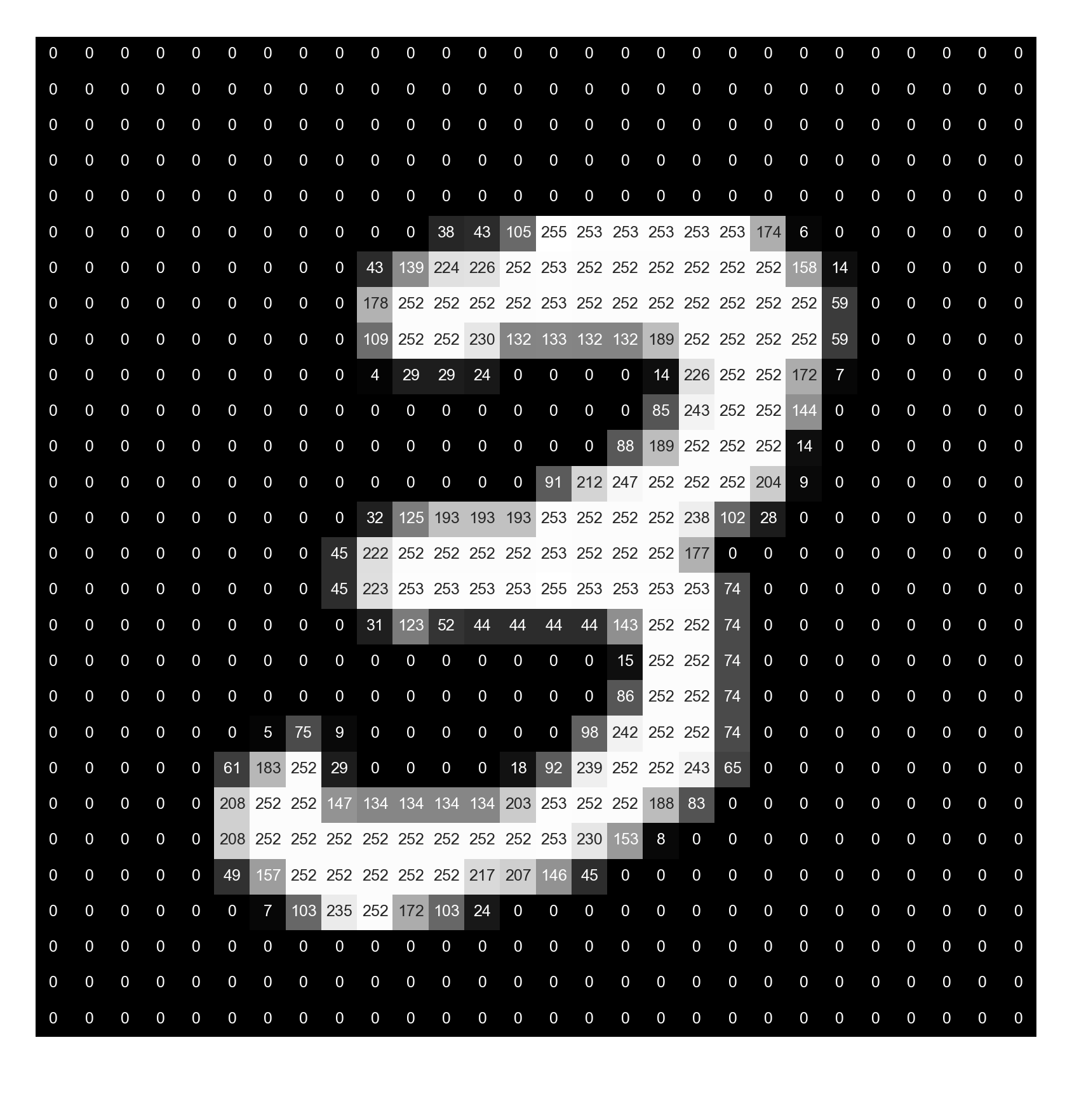
Let's start by training a fully connected model to predict which handwritten digit a 28 pixel by 28 pixel image contains. First we'll need to flatten out the image into a vector of 28x28 = 784 pixels, each represented as a number between 255 and 0. A value of 255 represents a white pixel and 0 a black one. The numbers in the middle of the range will represent different shades of grey.

1
from keras.datasets import mnist
2
from keras.models import Sequential
3
from keras.layers import Dense, Flatten, Activation
4
from keras.optimizers import SGD
5
from keras.utils import to_categorical
6
from matplotlib import pyplot as plt
7
import seaborn as sns
8

9
(x_train, y_train), (x_test, y_test) = mnist.load_data()
10

11
num_classes = 10
12

13
# Apply one-hot encoding to the labels
14
y_train = to_categorical(y_train, num_classes)
15
y_test = to_categorical(y_test, num_classes)
16

17
# Break training data into training and validation sets
18
(x_train, x_valid) = x_train[:50000], x_train[50000:]
19
(y_train, y_valid) = y_train[:50000], y_train[50000:]
20

21
# Model definition
22
model = Sequential()
23
model.add(Flatten(input_shape=(28,28)))
24

25
# Model hyperparameter
26
num_hidden_layers = 2
27
num_hidden_units = 10
28

29
for _ in range(num_hidden_layers):
30
    model.add(Dense(num_hidden_units))
31
    model.add(Activation('relu'))
32

33
# Output Layer
34
model.add(Dense(num_classes))
35
model.add(Activation('softmax'))
36

37
# Set optimization hyperparameters
38
batch_size = 256
39
epochs = 10
40

41
model.compile(optimizer='adam', loss='categorical_crossentropy',
42
    metrics=['accuracy'])
43

44
history = model.fit(x_train, y_train, epochs=epochs, batch_size=batch_size,
45
    validation_data=(x_valid, y_valid), verbose=2)
46

47
accuracy_score = model.evaluate(x_test, y_test, batch_size=128)
48

49
print(f'\nTest accuracy: {accuracy_score[1]:>5.3f}')
50

51
# Plot model accuracy and loss curves
52
plt.subplot(1,2,1)
53
plt.tight_layout()
54
plt.title('Accuracy')
55
plt.xlabel('Epochs')
56
plt.xticks(range(1, epochs+1, epochs//5))
57
plt.ylabel('Accuracy')
58
plt.plot(history.history['acc'], label='Training Accuracy')
59
plt.plot(history.history['val_acc'], label='Validation Accuracy')
60
plt.legend()
61

62
plt.subplot(1,2,2)
63
plt.tight_layout()
64
plt.plot(history.history['loss'], label='Training Loss')
65
plt.plot(history.history['val_loss'], label='Validation Loss')
66
plt.title('Loss')
67
plt.xlabel('Epochs')
68
plt.xticks(range(1, epochs+1, epochs//5))
69
plt.ylabel('Loss')
70
plt.legend()
71

72
plt.show()
73

On training the above model, we get the following results:

Epoch 1/10
1s - loss: 2.8814 - acc: 0.2122 - val_loss: 1.9508 - val_acc: 0.2677
Epoch 2/10
0s - loss: 1.9028 - acc: 0.2714 - val_loss: 1.8804 - val_acc: 0.2859
...
...
...
Epoch 10/10
0s - loss: 0.9046 - acc: 0.6434 - val_loss: 0.8798 - val_acc: 0.6495
 5632/10000 [===============>..............] - ETA: 0s
Test accuracy: 0.648

This is one of the simplest models we could have constructed and we get a final accuracy of 64.8%.

But how exactly can we judge that our model is too simple?

Bias and Variance

Two fundamental issues we need to keep in mind while training machine learning models are overfitting and underfitting.

Overfitting a model refers to the situation where a model "fits" extremely well to the training data. The model learns the feature representations of its training data and performs exceedingly well when asked to make predictions on the data it's seen before, but given a new data point, it falls flat. The usual culprit here is that we possibly allowed the model to train for longer than we should have. A model that overfits suffers from high variance.

On the other hand, Underfitting is the situation where our model fails to perform well on any data, training or testing. This happens when our model is not complex enough to capture the underlying relationships between the features and their true outputs.

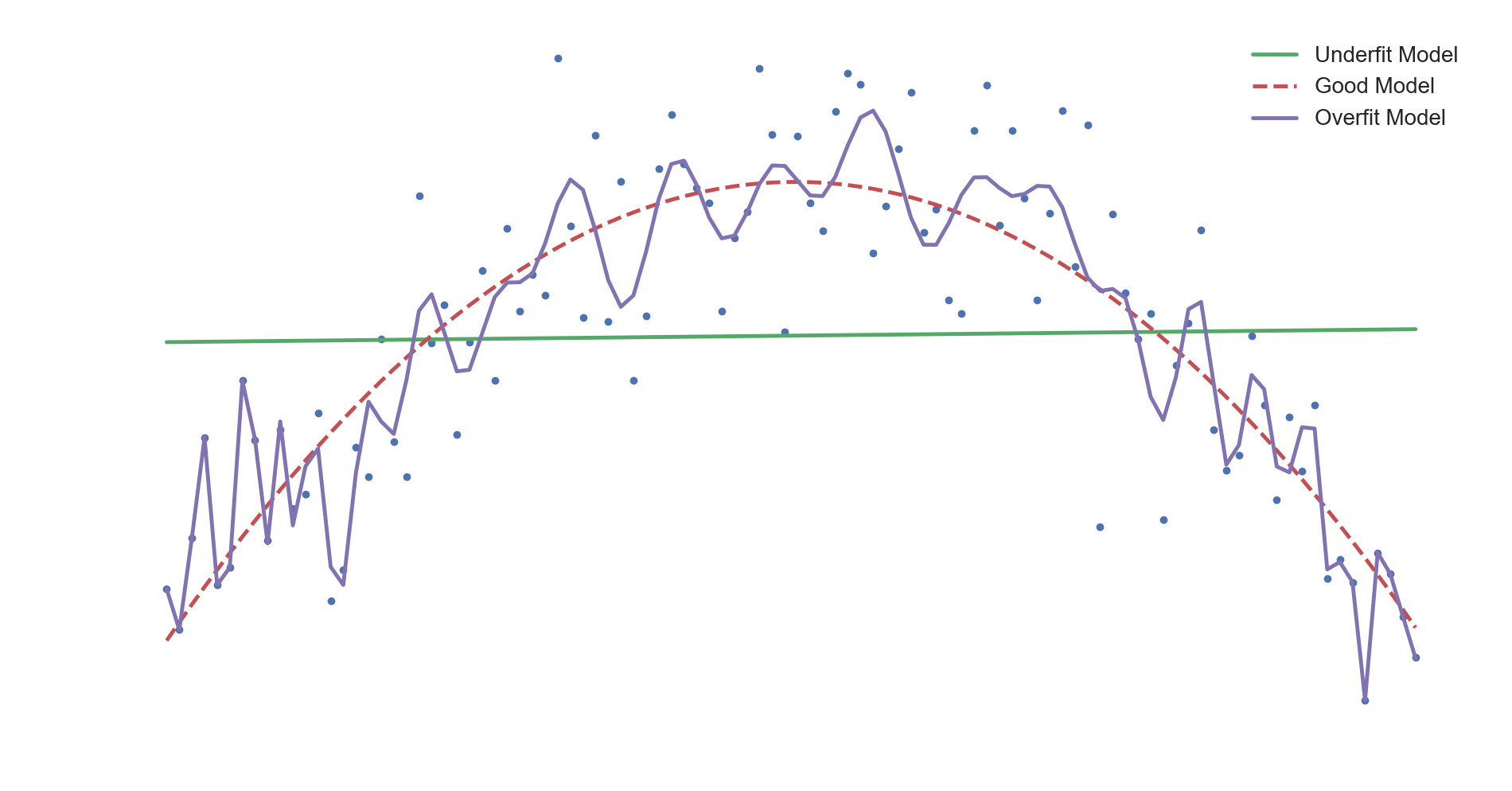
In the top figure above, we have training datapoints that are best approximated by an inverse parabola. A quadratic curve would be the best model for this dataset in terms of predictive performance. A linear model would be too simple to capture the pattern in the data and hence would underfit it, resulting in high model bias.

If we increase our model complexity, we would end up overfitting to the training data and the model would lose its ability to generalize well, which would be a case of high variance. This is seen in the above visualization, where as training progresses, the model tries to hit every single point in the dataset. We could see this as the model trying to fit itself to the noise fluctuations. It eventually loses it's ability to make accurate predictions on data it hasn't encountered before.

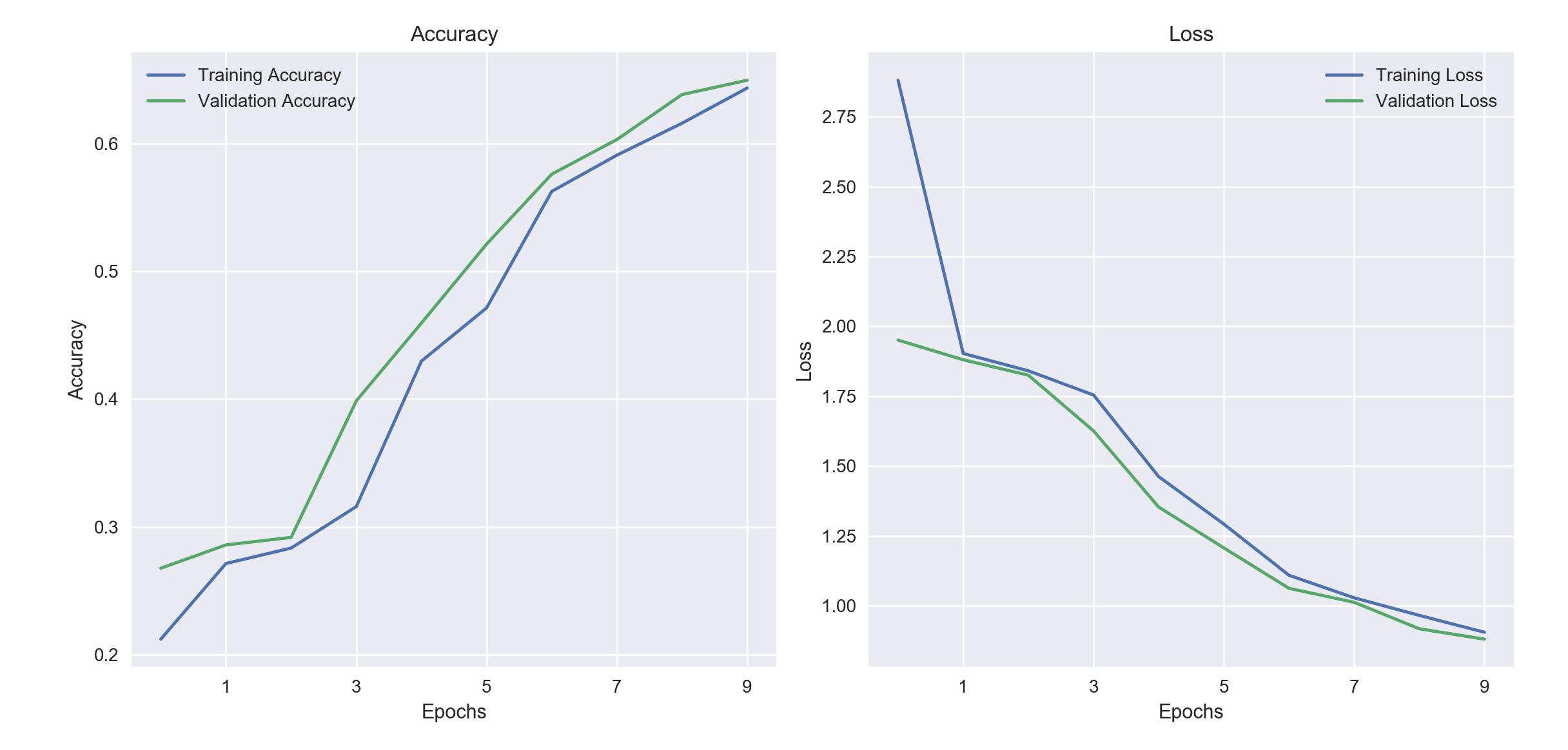
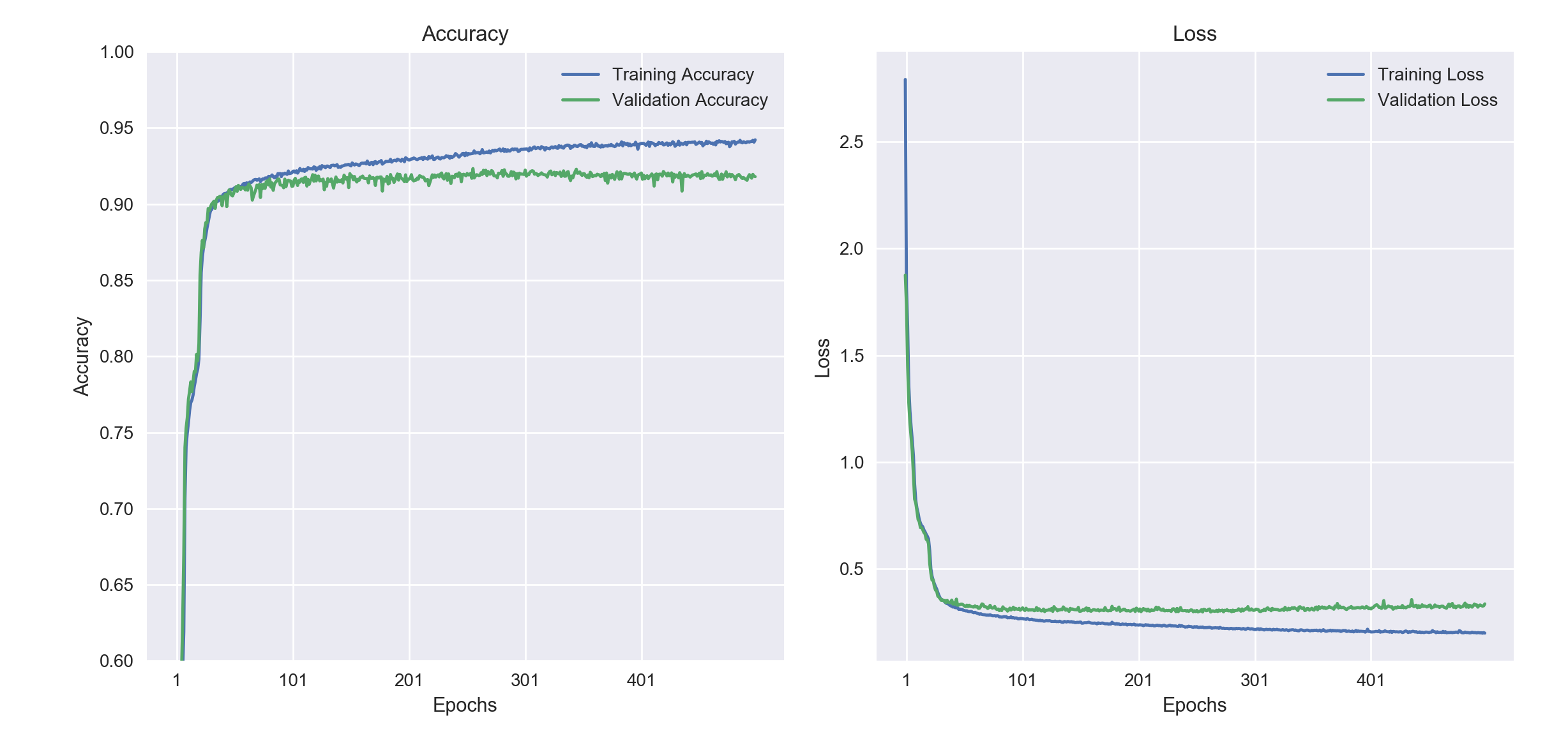
Now, in terms of model learning curves represented by the accuracy metric for our previously trained keras model, we see that the accuracy for both the training and the validation set follow each other closely. This suggests that we could train our model longer to observe increases in both training accuracy and validation accuracy. However, if we kept training our model, we would come to a point where the accuracy curves would start diverging. The training accuracy would keep on going up whereas the validation accuracy would plateau and might even go down. This is the point where we will have started to overfit our model and should stop the training process.

Below, we see how this plays out when we train the model for 500 epochs.

Increasing hidden layers and hidden units

To increase the representation power of our model, we increase the number of hidden layers and the number of hidden units in each of those layers. To begin with, let's see what happens when we increase the number of hidden units:

# Modifying relevant lines in previous code.
...
...
...
# Model definition
model = Sequential()
model.add(Flatten(input_shape=(28,28)))

# Model hyperparameter
num_hidden_layers = 2
num_hidden_units = 100

for _ in range(num_hidden_layers):
    model.add(Dense(num_hidden_units))
    model.add(Activation('relu'))
...
...
...

Train on 50000 samples, validate on 10000 samples
Epoch 1/10
1s - loss: 7.1802 - acc: 0.5452 - val_loss: 5.9891 - val_acc: 0.6232
Epoch 2/10
1s - loss: 6.0181 - acc: 0.6226 - val_loss: 5.7709 - val_acc: 0.6388
...
...
...
Epoch 10/10
1s - loss: 4.1331 - acc: 0.7408 - val_loss: 4.0006 - val_acc: 0.7492
 9984/10000 [============================>.] - ETA: 0s
Test accuracy: 0.741

Increasing the number of hidden units in the model's hidden layers lets the accuracy go upto 74.1%

How about if we kept the number of hidden units the same but increased the number of hidden layers?

...
...
...
# Model hyperparameter
num_hidden_layers = 10
num_hidden_units = 10

for _ in range(num_hidden_layers):
    model.add(Dense(num_hidden_units))
    model.add(Activation('relu'))
...
...
...

Train on 50000 samples, validate on 10000 samples
Epoch 1/10
3s - loss: 1.9715 - acc: 0.2329 - val_loss: 1.6083 - val_acc: 0.4083
Epoch 2/10
2s - loss: 1.3134 - acc: 0.5566 - val_loss: 1.0416 - val_acc: 0.6643
...
...
...
Epoch 10/10
2s - loss: 0.4021 - acc: 0.8916 - val_loss: 0.4129 - val_acc: 0.8948
 8064/10000 [=======================>......] - ETA: 0s
Test accuracy: 0.891

Increase the number of hidden layers resulted in much better performance! In practice, increasing the number of hidden layers gives us much higher performance than increasing the number of hidden units does.

Conclusion

In this post we explored the initial model iteration process. The number of hidden layers and the number of hidden units in those layers are the main model parameters to play around with when implementing a deep neural network.

In the next post we'll explore optimization hyperparameters like learning rate, batch size and epochs.