First steps with Apache Spark
2016-01-27
Introduction
For the past few months I've been hearing a lot about Spark and finally decided to see what it's all about. Having spent a few days playing around with a local setup, I think totally understandable why Spark has enjoyed such a rapid increase in popularity.
Not only is Spark extremely fast, it has awesome Python and R API's, which means that users can make use of REPL shells to perform real-time analysis on large datasets. Python and R already have rich ecosystems with active communities and Spark's support for these languages will most likely translate into these communities benefitting from and in turn contributing to the Spark Project. If you're familiar with SQL and Pandas for data analysis, Spark has SparkSQL and the Dataframes abstraction for working with structured data that will make you feel at home.
Background
The entire problem of analysing huge sets of data for a specific purpose was given a concrete form back in the early 2000's when Google needed an efficient way to implement its PageRank algorithm on the millions of webpages it crawled everyday. In two papers released by the company, a framework for distributed storage (The Google File System) and a paradigm for the distributed processing of data (MapReduce) were put forward as the solution.
These ideas led to the creation of Apache Hadoop which has since become the standard tool used by organizations to work with large scale data. But Hadoop has some serious limitations that Spark addresses nicely.
Hadoop requires data to be written to disk, which results in time-expensive operations that require you to execute a MapReduce job and sit back till it completes. Secondly, writing MapReduce jobs doesn't seem like a lot of fun for most programmers.
In comes Spark.
Spark was born out the AMPLab at UC Berkeley and open sourced by its developers. It aims to be a general processing engine that can work with HDFS data by utilizing in-memory computation, which makes it extremely fast. Further, Spark exposes high level API's in a number of languages including Python and R. This offers up a rich set of operations that can be implemented in a functional programming format. In this post, we'll explore Spark through its Python API.
Setup
There are a number of blog posts out there explaining how to get Spark up and running so I'll skip going over the procedure here. But a few pain-points that I faced post installation that aren't as widely covered so I'll highlight them here.
The first is to make sure that your SPARK_HOME environment variable is set correctly. I'm using Apache Spark version 1.5.2 on Mac OSX that I installed using Homebrew so SPARK_HOME corresponds to /usr/local/Cellar/apache-spark/1.5.2
export SPARK_HOME=/usr/local/Cellar/apache-spark/1.5.2
Since we'll be using IPython instead of the Pyspark shell, we need to make sure we can find the pyspark module in our import statement in IPython. Adding SPARK_HOME to the PYTHONPATH environment variable should do the job.
export PYTHONPATH=$SPARK_HOME/libexec/python:$SPARK_HOME/libexec/python/build:$PYTHONPATH
Finally, we'll be making use of the spark-csv package released by databricks to work with CSV files in Spark, so we need to make sure it is loaded during the SparkContext initialization.
export PACKAGES="com.databricks:spark-csv_2.11:1.3.0"
export PYSPARK_SUBMIT_ARGS="--packages ${PACKAGES} pyspark-shell"
For convenience, go ahead and put the above exports in your .zshrc or .bashrc file and source it (or just restart your terminal). We're also going to use ggplot for python for our visualizations.
pip install ggplot
Data
The dataset I chose for this post contains the info on all registered companies in India. It's available at https://data.gov.in/catalog/company-master-data It's a bit of work to download the data files individually as they sum up to about 300-400 mb of data. So if you'd rather just skip on working with the entire dataset, go ahead and download data on any two or more states and save the CSV's to a new folder.
While exploring the downloaded CSV's I noticed that not all of the data is in a standard format. Namely, the data for the state of Puducherry has some additional columns that will pose a problem while consolidating the data. So we'll keep it out of the analysis for now. Also, the header lines for some of the CSV's contain additional whitespaces that we should collapse before reading in just to be sure we won't be tripped up later on.
find . -type f -name "*.csv" -execdir sed -i.bk '1s/ *//g' {} \;
The above command finds all the CSV files in the current directory and passes them to the sed utility which collapses all whitespaces in the first line of each file while making backups of the file. So when it finishes, you'll find a whole bunch of backup files in your directory with the extension ".bk".
We're all set to start analysing the data. Go ahead and start an IPython session.
We need to perform the necessary imports to get a SparkContext running and initialize it with 2 cores.
from pyspark import SparkContext
from pyspark import SQLContext

sc = SparkContext('local[2]')
sqlct = SQLContext(sc)
Now, in our current directory, we have several csv files with a common schema. To perform any sort of analysis on all this data at once, it's necessary for us to consolidate this data into a single RDD (Resilient Distributed Dataset), which is Spark's main abstraction for working with data. We'll follow a two step procedure where we first read in the CSV's individually into their respective dataframes and then concatenate them all into a single dataframe.
from glob import glob
from os.path import abspath

# List all files in the current directory and convert them into their absolute paths.
filenames = map(lambda x: abspath(x), glob('*.csv'))

# Read in CSV's into individual Spark dataframes and hold them in a list.
frames = map(lambda x: \
           sqlct.read.format('com.databricks.spark.csv').\
           options(header="true", inferschema="false").\
           load(x), filenames)

# Reduce individual frames to a single concatenated frame.
companies = reduce(lambda x, y: x.unionAll(y), frames)
The above operations are unnecessary because the Spark-CSV API accepts glob by default. Nevertheless, the above code was useful in explaining how individual dataframes can be concatenated if the need be. Here's how it could've been in a single line.
companies = sqlct.read.format('com.databricks.spark.csv').\
                            options(header = "true", inferschema = "false").\
                            load('*.csv')
Now that we have all the CSV data on the different states in a Spark dataframe. Let's perform some basic analysis.
# Count the number of records in our dataset
companies.count()
#
# 1377813


# Explore the schema of our dataset.
companies.printSchema()
#
#  root
# |-- CORPORATE_IDENTIFICATION_NUMBER: string (nullable = true)
# |-- DATE_OF_REGISTRATION: string (nullable = true)
# |-- COMPANY_NAME: string (nullable = true)
# |-- COMPANY_STATUS: string (nullable = true)
# |-- COMPANY_CLASS: string (nullable = true)
# |-- COMPANY_CATEGORY: string (nullable = true)
# |-- AUTHORIZED_CAPITAL: string (nullable = true)
# |-- PAIDUP_CAPITAL: string (nullable = true)
# |-- REGISTERED_STATE: string (nullable = true)
# |-- REGISTRAR_OF_COMPANIES: string (nullable = true)
# |-- PRINCIPAL_BUSINESS_ACTIVITY: string (nullable = true)
# |-- REGISTERED_OFFICE_ADDRESS: string (nullable = true)
# |-- SUB_CATEGORY: string (nullable = true)


# Print first 10 records
companies.show(10)


# Show distinct values taken on by the COMPANY_STATUS column
companies.select('COMPANY_STATUS').distinct().show()
#
# +--------------------+
# |      COMPANY_STATUS|
# +--------------------+
# |             DEFAULT|
# |UNDER PROCESS OF ...|
# |              ACTIVE|
# |         AMALGAMATED|
# |  ACTIVE IN PROGRESS|
# |Dormant under sec...|
# |          STRIKE OFF|
# |             DORMANT|
# |   UNDER LIQUIDATION|
# |          LIQUIDATED|
# |CONVERTED TO LLP ...|
# |    CONVERTED TO LLP|
# |           DISSOLVED|
# +--------------------+


# Count the number of companies that have COMPANY_STATUS as 'ACTIVE'
companies.filter(companies.COMPANY_STATUS == 'ACTIVE').count()
#
# 966855
Spark SQL
The Spark SQL module provides an additional way to work with structured data. This means that even if you're not too familiar with Pandas dataframes but have a background in SQL, you're good to go.
Spark Dataframes are conceptually the same as tables in a relational database, which allows SQL queries to be run on them. To analyze the data using SQL queries, we first need to initialize the SQLContext and register our Dataframe as a table.
from pyspark import SQLContext

# Initialize SQLContext
sqlct = SQLContext(sc)

# Register the Dataframe
companies.registerTempTable('companies')
Queries can be executed by using the 'sql' module of our SQLContext. Keep in mind that SQL queries return Dataframes themselves, so to see the actual result we'll need to call the show() method on them.
# Count the number of records
sqlct.sql('SELECT COUNT(*) as total_companies FROM companies').show()
#
# +---------------+
# |total_companies|
# +---------------+
# |        1377813|
# +---------------+


# Describe the table schema
sqlct.sql('DESCRIBE companies').show(truncate = False)
#
# +-------------------------------+---------+-------+
# |col_name                       |data_type|comment|
# +-------------------------------+---------+-------+
# |CORPORATE_IDENTIFICATION_NUMBER|string   |       |
# |DATE_OF_REGISTRATION           |string   |       |
# |COMPANY_NAME                   |string   |       |
# |COMPANY_STATUS                 |string   |       |
# |COMPANY_CLASS                  |string   |       |
# |COMPANY_CATEGORY               |string   |       |
# |AUTHORIZED_CAPITAL             |string   |       |
# |PAIDUP_CAPITAL                 |string   |       |
# |REGISTERED_STATE               |string   |       |
# |REGISTRAR_OF_COMPANIES         |string   |       |
# |PRINCIPAL_BUSINESS_ACTIVITY    |string   |       |
# |REGISTERED_OFFICE_ADDRESS      |string   |       |
# |SUB_CATEGORY                   |string   |       |
# +-------------------------------+---------+-------+


# Performing Aggregations
# Let's see the top 10 states according to the count of the companies registered.
sqlct.sql('SELECT REGISTERED_STATE, COUNT(*) AS count FROM companies \
          GROUP BY REGISTERED_STATE \
          ORDER BY count DESC \
          LIMIT 10').show()
#
# +----------------+------+
# |REGISTERED_STATE| count|
# +----------------+------+
# |     Maharashtra|294705|
# |           Delhi|272369|
# |     West Bengal|185052|
# |      Tamil Nadu|114428|
# |         Gujarat| 81184|
# |       Telangana| 77040|
# |   Uttar Pradesh| 65165|
# |       Rajasthan| 45804|
# |          Kerala| 37905|
# |  Madhya Pradesh| 29782|
# +----------------+------+


# The above SQL query can also be exececuted as through the Dataframe API.
companies.groupby('REGISTERED_STATE').count().sort('count', ascending=False).show(10)
#
# +----------------+------+
# |REGISTERED_STATE| count|
# +----------------+------+
# |     Maharashtra|294705|
# |           Delhi|272369|
# |     West Bengal|185052|
# |      Tamil Nadu|114428|
# |         Gujarat| 81184|
# |       Telangana| 77040|
# |   Uttar Pradesh| 65165|
# |       Rajasthan| 45804|
# |          Kerala| 37905|
# |  Madhya Pradesh| 29782|
# +----------------+------+
As we can see, Spark provides a rich and flexible set of APIs that can be implemented according to the user's preference.
Now let's see how new businesses have been set up over the years in India.
We have a DATE_OF_REGISTRATION column in our dataset. A bar plot of the number of new businesses registered in India every year would definitely make for an interesting visualization. Let's create a new YEAR_OF_REGISTRATION column in our Dataframe that we will derive from the DATE_OF_REGISTRATION column.
To extract the year from the date, we will have to define a custom function.
# If date has format dd-mm-YYYY, then split on '-' and return YYYY, otherwise return 0

def extract_year(date):
    if "-" in date:
        return int(date.split("-")[2])
    else:
        return 0
The above function will be passed as a UserDefinedFunction when we create a new dataframe.
from pyspark.sql.dataframe import IntegerType
from pyspark.sql.functions import UserDefinedFunction

udf = UserDefinedFunction(extract_year, IntegerType())

# Create new Dataframe with YEAR_OF_REGISTRATION column.
companies = companies.withColumn('YEAR_OF_REGISTRATION', udf(companies.DATE_OF_REGISTRATION))

companies.printSchema()
#
#  root
# |-- CORPORATE_IDENTIFICATION_NUMBER: string (nullable = true)
# |-- DATE_OF_REGISTRATION: string (nullable = true)
# |-- COMPANY_NAME: string (nullable = true)
# |-- COMPANY_STATUS: string (nullable = true)
# |-- COMPANY_CLASS: string (nullable = true)
# |-- COMPANY_CATEGORY: string (nullable = true)
# |-- AUTHORIZED_CAPITAL: string (nullable = true)
# |-- PAIDUP_CAPITAL: string (nullable = true)
# |-- REGISTERED_STATE: string (nullable = true)
# |-- REGISTRAR_OF_COMPANIES: string (nullable = true)
# |-- PRINCIPAL_BUSINESS_ACTIVITY: string (nullable = true)
# |-- REGISTERED_OFFICE_ADDRESS: string (nullable = true)
# |-- SUB_CATEGORY: string (nullable = true)
# |-- YEAR_OF_REGISTRATION: integer (nullable = true)
Now we aggregate the records by YEAR_OF_REGISTRATION and coerce our Spark Dataframe to a Pandas Dataframe, which we will need to create a visualization with ggplot.
year_formed = companies.\
  filter('YEAR_OF_REGISTRATION < 2016').\
  filter('YEAR_OF_REGISTRATION > 1980').\
  groupby('YEAR_OF_REGISTRATION').\
  count().\
  orderBy('YEAR_OF_REGISTRATION', ascending=True).toPandas()

# Let's not forget to import the ggplot functionality!
from ggplot import *

# Plot bar graph of No. of companies registered per year since 1980.
plot = ggplot(aes(x="YEAR_OF_REGISTRATION", y="count"), data=year_formed) + \
  geom_bar(stat="identity", colour="black", fill="orange") + \
  xlab('Year') + \
  ylab('No. of Companies formed') + \
  scale_x_discrete(breaks=range(1979, 2016, 2)) + \
  xlim(1980, 2016)

# Save graph to file
ggsave(plot, "companies_plot.png", width=15, height=8)
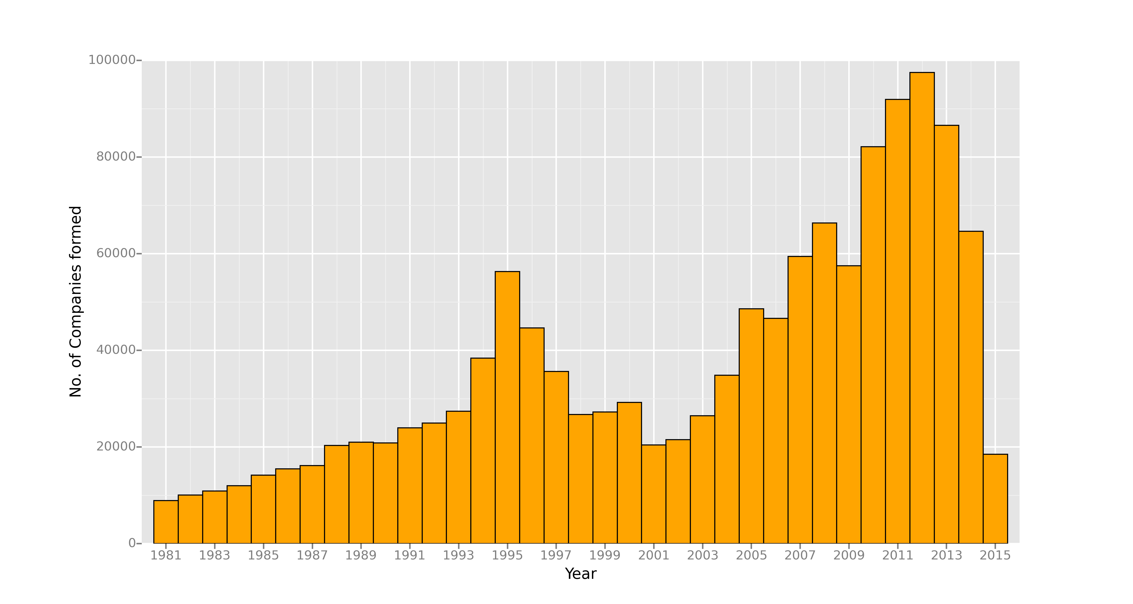
The registrations pattern is clearly not uniform. There was quite a noticeable peak in new company registrations in 1995, which dwindled to less than half that number over the next 5 years, picking up again for a decade long growth spurt which has again tumbled down over the past couple of years.
Note that we only have data uptill March of 2015.
We can explore our data further to gain a deeper understanding of what's driven such a trend. But since this post is about exploring Spark functionality let's stop here and leave the analysis to another post.
Conclusion
I hope that I was able to explain some of Spark's features well enough for you to start working with it yourself.
The dataframes API and SparkSQL make it a breeze to work with structured data while leveraging the benefits of fast and
distributed processing.
Spark is under rapid development and already has 100's of contributers actively involved in the project.
More functionality, language support and high level operations are being added with every new release which is driving
Spark's rapid adoption in industry.