Batch Normalization in deep neural networks.
2017-08-10
Batch Normalization is a straightforward way for optimizing the training of deep neural networks. It is based on the idea that inputs to all layers of a neural network should be whitened - i.e. linearly transformed to have zero mean and unit variance, before being fed into the activation function. This results in eliminating the effects of what the authors of the paper introducing this technique call "Internal Covariate Shift", which is the change in the distributions of each of the layer activations as we move forward in a network.
The term "Covariate Shift" refers to a change in the input distribution to any learning system and can be attributed to Shimodaira, 2000. When we consider a deep neural network not as a singular learning system, but as a composition of trainable layers, we can apply the concept of covariate shift to all the layers in the network.
Let's explore the 2015 paper by Sergey Ioffe and Christian Szegedy, introducing the batch normalization technique further.
The problem
While training deep neural networks, the distribution of each layer's inputs changes as the parameters of the previous layers are updated. This covariate shift becomes an issue especially in deep neural nets with many layers as we end up constrained with lower learning rates and extremely sensitive parameter initialization strategies. Another challenge that presents itself is when working with saturating non-linearities like the tanh non-linearity.
To see how this can be a problem let's evaluate the statistics of the activations in a simple feed-forward neural net with 10 hidden layers containing 200 nodes each.
1 # Code adapted from Andrej Karpathy's CS231n slides.
2
3 import numpy as np
4 import seaborn as sns
5 from matplotlib import pyplot as plt
6
7 inputs = np.random.randn(500, 200)
8 hidden_layers = [200] * 10
9 nonlinearities = ['tanh']*len(hidden_layers)
10
11 activations = {
12 'relu': lambda x:np.maximum(0, x),
13 'tanh': lambda x:np.tanh(x)}
14
15 hidden_activations = {}
16
17 for i in range(len(hidden_layers)):
18 X = inputs if i == 0 else hidden_activations[i-1]
19 fan_in = X.shape[1]
20 fan_out = hidden_layers[i]
21
22 #W = np.random.randn(fan_in, fan_out) / np.sqrt(fan_in) # Xavier Init
23 W = np.random.randn(fan_in, fan_out) * 0.01 # Normal init
24
25 H = np.dot(X, W)
26 H = activations[nonlinearities[i]](H)
27
28 hidden_activations[i] = H
29
30
31 layer_means = [np.mean(H) for i, H in hidden_activations.items()]
32 layer_stds = [np.std(H) for i, H in hidden_activations.items()]
33
34 plt.figure()
35 plt.subplot(121)
36 plt.plot(list(hidden_activations.keys()), layer_means, 'ob-')
37 plt.title('layer mean')
38 plt.subplot(122)
39 plt.plot(list(hidden_activations.keys()), layer_stds, 'or-')
40 plt.title('layer std')
41
42 fig = plt.figure()
43 for i, H in hidden_activations.items():
44 ax = plt.subplot(1, len(hidden_activations), i+1)
45 ax.hist(H.ravel(), 30, range=(-1,1))
46 ax.grid(True)
47 for tic in ax.yaxis.get_major_ticks():
48 tic.tick1On = tic.tick2On = False
49 tic.label1On = tic.label2On = False
50 plt.title('Layer: %s \nMean: %1.4f\nStd: %1.6f' % (
51 i+1, layer_means[i], layer_stds[i]), fontsize=10)
52
The code above produces the following two graphs:
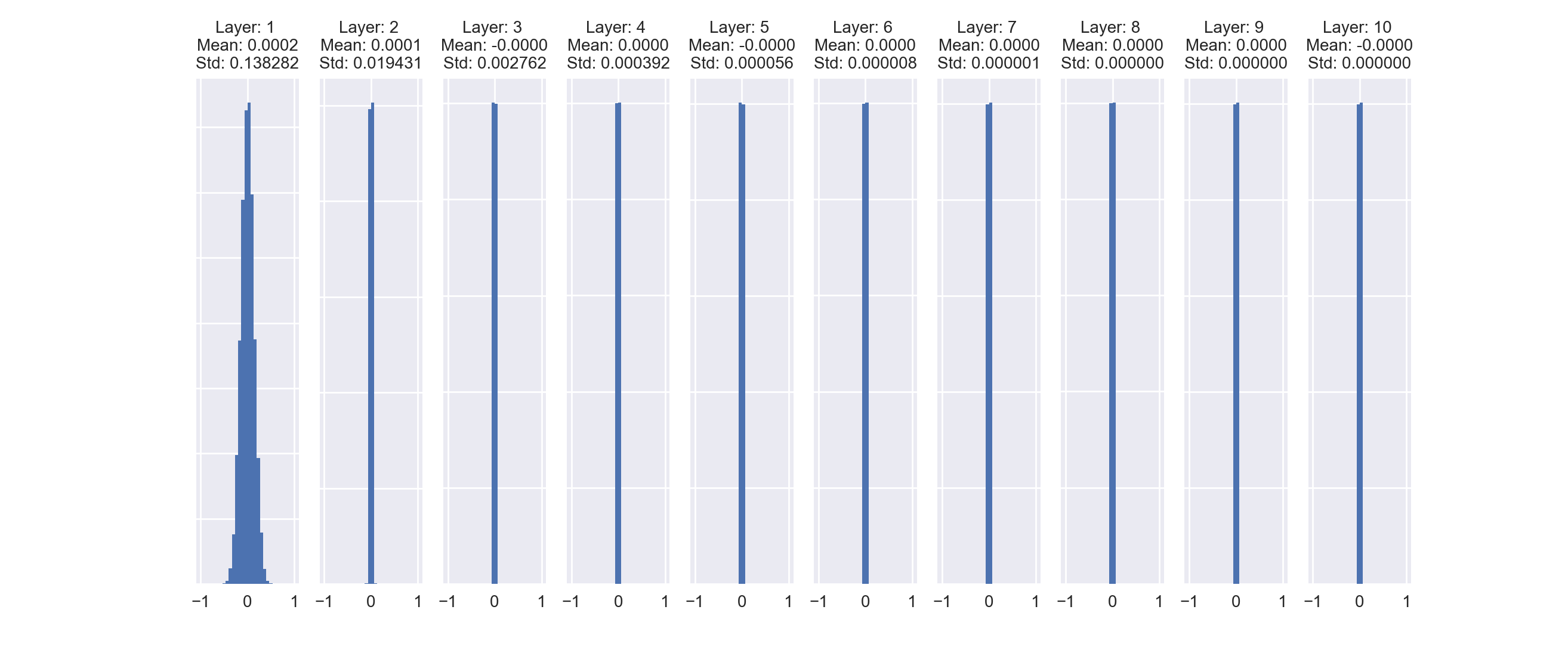
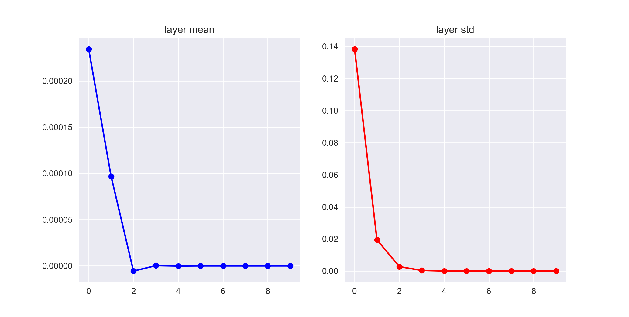
As we see in the higher layers, the distribution becomes highly concentrated around the mean as the standard deviation of the layer activations plummets. These near-zero activations subsequently lead to very small gradients during backpropagation that make it extremely difficult to train the network efficiently.
One of the ways we deal with this problem is by carefully initializing the model parameters. Glorot et. al suggested using the xavier initialization which corresponds to the weight matrix in the above code to be initialized as W = np.random.randn(fan_in, fan_out) / np.sqrt(fan_in). Using this initialization strategy, our layer activation statistics look like the following.
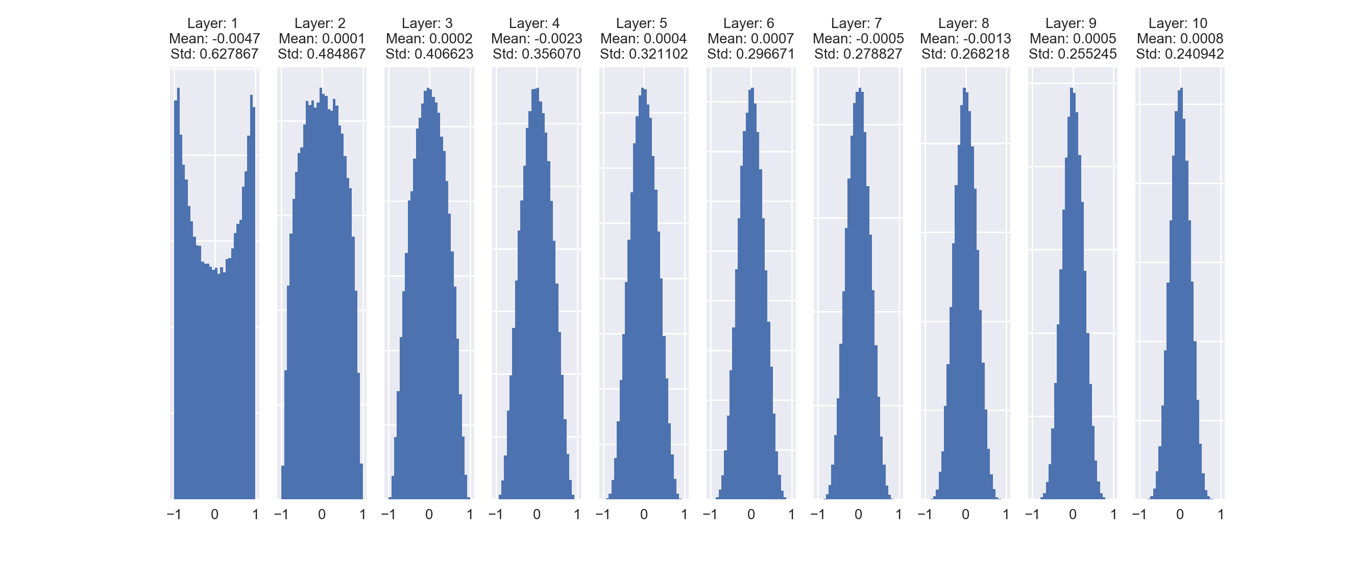
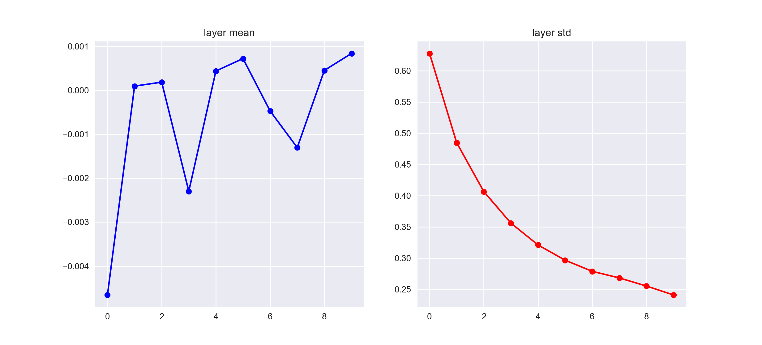
Although the standard deviations of the layer activations are still decreasing, they are doing so at a much more reasonable rate, which allows our network to train efficiently even for deeper architectures.
Batch Normalization solves this problem by transforming activations across all the layers to unit gaussian activations. This takes care of the issue of internal covariate shift and results in a number of benefits for our network such as:
- Reduced training time. (due to improved gradient flow through the network)
- The capability to handle higher learning rates. (which helps with fast convergence)
- Acting as a model regularizer (All training examples in a batch get tied together due to batch normalization. This tends to have an overall regularizing effect)
- Reducing the dependency on proper weights initialization.
- Making saturating non-linearities viable options for use as activation functions.
The mechanics of Batch Normalization
In their paper, the authors normalize each scalar feature independently, by making the mean 0 and variance 1. If a layer has \(d\) inputs with the corresponding input vector as \(x = (x^{(1)}...x^{(d)})\), each dimension will be normalized as the following, with expectation and variance being computed over the training data set. $$\hat{x}^{(k)} = \frac{x^{(k)} - E[x^{(k)}]}{\sqrt{Var[x^{(k)}]}}$$
Simply normalizing each input of a layer can restrict the representational power of the network. To address this, we have to allow the network to learn to undo the batch normalization transform by making sure the transformation can represent the identity transform. This is achieved by introducing a pair of parameters \(\gamma^{(k)},\beta^{(k)}\) for each activation \(x^{(k)}\) that can, respectively, scale and shift the normalized values as necessary (\(\gamma^{(k)}\) and \(\beta^{(k)}\) are learnable/trainable parameters)
With the above scale and shift parameters in hand, each normalized activation \(\hat{x}^{(k)}\) can be viewed as an input to a sub-network composed of the linear transformation: $$y^{(k)} = \gamma^{(k)}\hat{x}^{(k)} + \beta^{(k)} $$ followed by the later processing done by the original network.
As mentioned, \(\gamma^{(k)}\) and \(\beta^{(k)}\) can be learned alongwith the model weights and serve to restore the representational power of the network. This can be seen if we set \(\gamma^{(k)} = \sqrt{Var[x^{(k)}]}\) and \(\beta^{(k)} = E[x^{(k)}]\). This way the model can recover the original activations if it learned that to be the optimal behaviour.
In practice, for any given mini-batch the normalization transformation is applied to each input dimension (activation) independently, with the activation first undergoing normalization (\(\hat{x}\)) and then a linear transformation (\(y\)).
For a mini-batch \(B\) of size \(m\),
$$ \mu_{B} = \frac{1}{m}\sum_{i=1}^{m}x_{i} $$
$$ \sigma_{B}^{2} = \frac{1}{m}\sum_{i=1}^{m}(x_{i} - \mu_{B})^{2} $$
$$ \hat{x_{i}} = \frac{x_i - \mu_B}{\sqrt{\sigma_B^2 + \epsilon}} $$
$$ y_{i} = \gamma\hat{x_{i}} + \beta \equiv BN(x_{i}) $$
where, \(y_{i}\) is the Batch Normalizing Transform \(BN(x_{i})\), \(\hat{x_{i}}\) is the normalized activation and the values \(\mu_{B}\) and \(\sigma_{B}^2\) are the mini-batch mean and mini-batch variance respectively. Note: the value \(\epsilon\) is a small constant added for numerical stability to make sure we do not perform any divide-by-zero operations.
Tensorflow implementation
Let's construct a deep neural network with 10 hidden layers containing 100 nodes each. We need to make sure that the initial weights for both the networks, with and without batch normalization are the same.
The tensorflow API handles downloading the MNIST dataset, extracting it, and preprocessing it into the right form for us. While constructing the computational graph for both models, the main implementation difference comes up while constructing the individual layers.
Normally we'd contruct a network layer by matrix multiplying the weights and the input tensors and then adding the bias values. For batch normalization, all of the above math implementations are handled for us by the tf.layers.batch_normalization API. If we wanted lower level control over the mechanics of the implementation, we could use the tf.nn.batch_normalization function instead (which would be a lot more work).
Note: We implement batch normalization before the output is fed into the activation function. We also don't explicitly add bias here because it's role is performed by the \(\beta\) variable. For details see Section 3.2 of the original paper.
1 import tensorflow as tf
2 import tqdm
3 import numpy as np
4 import seaborn as sns # for nice looking graphs
5 from matplotlib import pyplot as plt
6
7 from tensorflow.examples.tutorials.mnist import input_data
8 mnist = input_data.read_data_sets("MNIST_data/", one_hot=True)
9
10 np.random.seed(42)
11
12 def create_layer(
13 input_tensor,
14 weight,
15 name,
16 activation,
17 training=None):
18 w = tf.Variable(weight)
19 b = tf.Variable(tf.zeros([weight.shape[-1]]))
20 z = tf.add(tf.matmul(input_tensor, w), b, name='layer_input_%s' % name)
21 if name == 'output':
22 return z, activation(z, name='activation_%s' % name)
23 else:
24 return activation(z, name='activation_%s' % name)
25
26 def create_batch_norm_layer(
27 input_tensor,
28 weight,
29 name,
30 activation,
31 training):
32 w = tf.Variable(weight)
33 linear_output = tf.matmul(input_tensor, w)
34 batch_norm_z = tf.layers.batch_normalization(
35 linear_output, training=training, name='bn_layer_input_%s' % name)
36 if name == 'output':
37 return batch_norm_z, activation(batch_norm_z, name='bn_activation_%s' % name)
38 else:
39 return activation(batch_norm_z, name='bn_activation_%s' % name)
40
41 def get_tensors(
42 layer_creation_fn,
43 inputs,
44 labels,
45 weights,
46 activation,
47 learning_rate,
48 is_training):
49 l1 = layer_creation_fn(inputs, weights[0], '1', activation, training=is_training)
50 l2 = layer_creation_fn(l1, weights[1], '2', activation, training=is_training)
51 l3 = layer_creation_fn(l2, weights[2], '3', activation, training=is_training)
52 l4 = layer_creation_fn(l3, weights[3], '4', activation, training=is_training)
53 l5 = layer_creation_fn(l4, weights[4], '5', activation, training=is_training)
54 l6 = layer_creation_fn(l5, weights[5], '6', activation, training=is_training)
55 l7 = layer_creation_fn(l6, weights[6], '7', activation, training=is_training)
56 l8 = layer_creation_fn(l7, weights[7], '8', activation, training=is_training)
57 l9 = layer_creation_fn(l8, weights[8], '9', activation, training=is_training)
58 logits, output = layer_creation_fn(
59 l9, weights[9], 'output', tf.nn.sigmoid, training=is_training)
60
61 cross_entropy = tf.reduce_mean(
62 tf.nn.softmax_cross_entropy_with_logits(labels=labels, logits=logits))
63
64 correct_prediction = tf.equal(tf.argmax(output, 1), tf.argmax(labels, 1))
65 accuracy = tf.reduce_mean(tf.cast(correct_prediction, tf.float32))
66
67 if layer_creation_fn.__name__ == 'create_batch_norm_layer':
68 with tf.control_dependencies(tf.get_collection(tf.GraphKeys.UPDATE_OPS)):
69 optimizer = tf.train.GradientDescentOptimizer(
70 learning_rate).minimize(cross_entropy)
71 else:
72 optimizer = tf.train.GradientDescentOptimizer(
73 learning_rate).minimize(cross_entropy)
74
75 return accuracy, optimizer
76
77
78 def train_network(
79 learning_rate_val,
80 num_batches,
81 batch_size,
82 activation,
83 bad_init=False,
84 plot_accuracy=True):
85
86 inputs = tf.placeholder(tf.float32, shape=[None, 784], name='inputs')
87 labels = tf.placeholder(tf.float32, shape=[None, 10], name='labels')
88 learning_rate = tf.placeholder(tf.float32, name='learning_rate')
89 is_training = tf.placeholder(tf.bool, name='is_training')
90
91 np.random.seed(42)
92
93 scale = 1 if bad_init else 0.1
94
95 weights = [
96 np.random.normal(size=(784, 100), scale=scale).astype(np.float32),
97 np.random.normal(size=(100, 100), scale=scale).astype(np.float32),
98 np.random.normal(size=(100, 100), scale=scale).astype(np.float32),
99 np.random.normal(size=(100, 100), scale=scale).astype(np.float32),
100 np.random.normal(size=(100, 100), scale=scale).astype(np.float32),
101 np.random.normal(size=(100, 100), scale=scale).astype(np.float32),
102 np.random.normal(size=(100, 100), scale=scale).astype(np.float32),
103 np.random.normal(size=(100, 100), scale=scale).astype(np.float32),
104 np.random.normal(size=(100, 100), scale=scale).astype(np.float32),
105 np.random.normal(size=(100, 10), scale=scale).astype(np.float32)]
106
107 vanilla_accuracy, vanilla_optimizer = get_tensors(
108 create_layer,
109 inputs,
110 labels,
111 weights,
112 activation,
113 learning_rate,
114 is_training)
115
116 bn_accuracy, bn_optimizer = get_tensors(
117 create_batch_norm_layer,
118 inputs,
119 labels,
120 weights,
121 activation,
122 learning_rate,
123 is_training)
124
125 vanilla_accuracy_vals = []
126 bn_accuracy_vals = []
127
128 with tf.Session() as sess:
129 sess.run(tf.global_variables_initializer())
130
131 for i in tqdm.tqdm(list(range(num_batches))):
132 batch_xs, batch_ys = mnist.train.next_batch(batch_size)
133
134 sess.run([vanilla_optimizer], feed_dict={
135 inputs: batch_xs,
136 labels: batch_ys,
137 learning_rate: learning_rate_val,
138 is_training: True})
139
140 sess.run([bn_optimizer], feed_dict={
141 inputs: batch_xs,
142 labels: batch_ys,
143 learning_rate: learning_rate_val,
144 is_training: True})
145
146 if i % batch_size == 0:
147 vanilla_acc = sess.run(vanilla_accuracy, feed_dict={
148 inputs: mnist.validation.images,
149 labels: mnist.validation.labels,
150 is_training: False})
151
152 bn_acc = sess.run(bn_accuracy, feed_dict={
153 inputs: mnist.validation.images,
154 labels: mnist.validation.labels,
155 is_training: False})
156
157 vanilla_accuracy_vals.append(vanilla_acc)
158 bn_accuracy_vals.append(bn_acc)
159
160 print(
161 'Iteration: %s; ' % i,
162 'Vanilla Accuracy: %2.4f; ' % vanilla_acc,
163 'BN Accuracy: %2.4f' % bn_acc)
164
165 if plot_accuracy:
166 plt.title('Training Accuracy')
167 plt.plot(range(0, len(vanilla_accuracy_vals) * batch_size, batch_size),
168 vanilla_accuracy_vals, label='Vanilla network')
169 plt.plot(range(0, len(bn_accuracy_vals) * batch_size, batch_size),
170 bn_accuracy_vals, label='Batch Normalized network')
171 plt.tight_layout()
172 plt.legend()
173 plt.grid(True)
174 plt.show()
175
176
We'll run the train_network function and pass in different model parameters to compare how the network performs with and without batch normalization.
To begin with, let's start with a reasonable learning rate and the tanh non-linearity as our activation function.
train_network(0.01, 2000, 60, tf.nn.tanh)
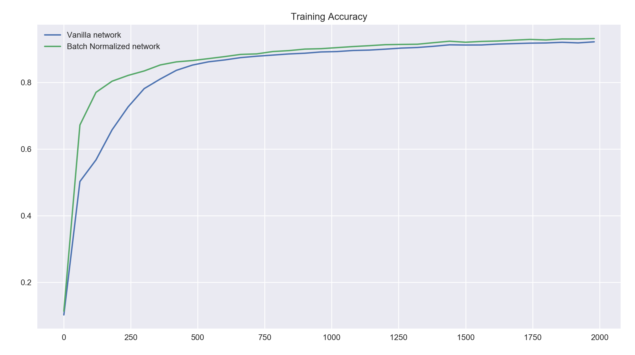
We see that both networks perform reasonably well but the batch normalized network achieves a high accuracy much faster than our vanilla network. It maintains a slightly higher accuracy value for further iterations of batches. Both the networks would probably converge to a higher accuracy value if trained further.
Next, we train our networks similarly to the previous networks but this time, we initialize the weights to these networks sub-optimally. In practice, using zero-centered, small initial weight values give much better results for neural networks. Here, we sample the initial weights from a normal distribution with standard deviation of 1 (the weights in the previous experiment were initialized with a standard deviation of 0.1).
train_network(0.01, 5000, 60, tf.nn.tanh, bad_init=True)
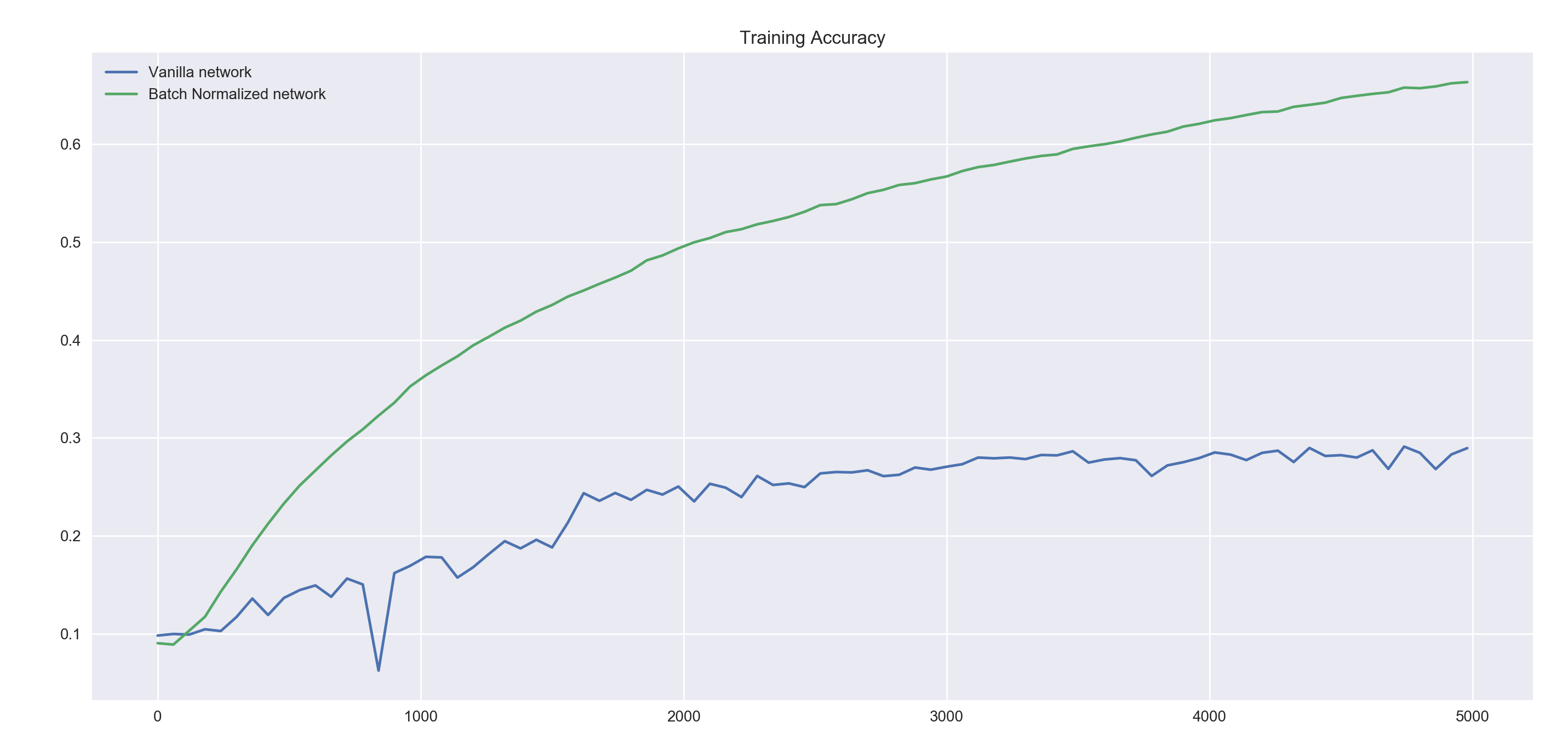
We see that even with 5000 iterations, both networks perform much worse than our previous networks but even here the batch normalized network performs much better than our vanilla network. Notice the lower volatility displayed by the accuracy of the batch normalized network.
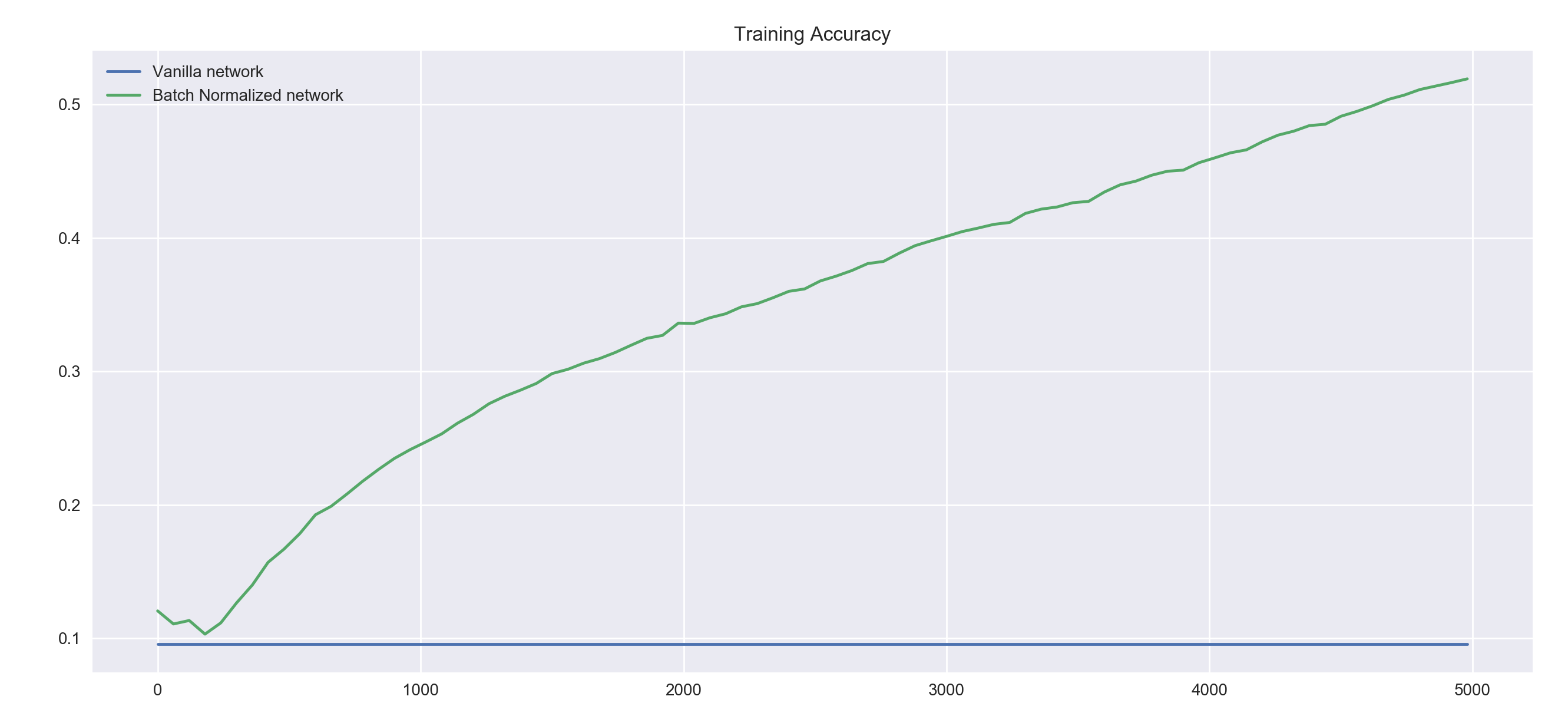
Next, we not don't just initialize the networks with bad weights, we also pass in an extremely high learning rate of 1. This learning rate is a hundred times the one we used in the previous runs.
train_network(1, 5000, 60, tf.nn.tanh, bad_init=True)
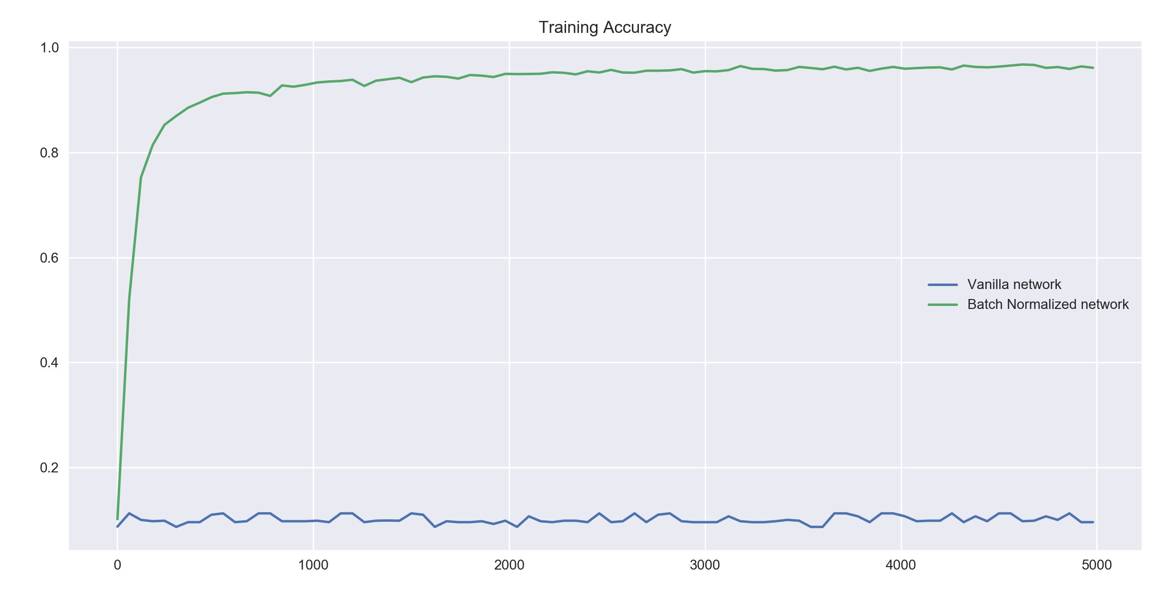 As expected, our vanilla neural network doesn't even get off the ground. The accuracy remains somewhere around 0.1 or 10 percent, which given 10 output classes to predict from, is as good as random guessing.
The batch normalized network however performs extremely well here. Even though the bad initial weights bog it down just the same as the vanilla network, it does really well when passed a high learning rate, leading to convergence at a high accuracy.
Let's try a different non-linearity next.
train_network(0.01, 2000, 60, tf.nn.relu)
 For the ReLu non-linearity and a relatively small iteration limit of 2000 batches, both networks end up giving similar accuracies but the batch normalized network gets there faster and with much less volatility.
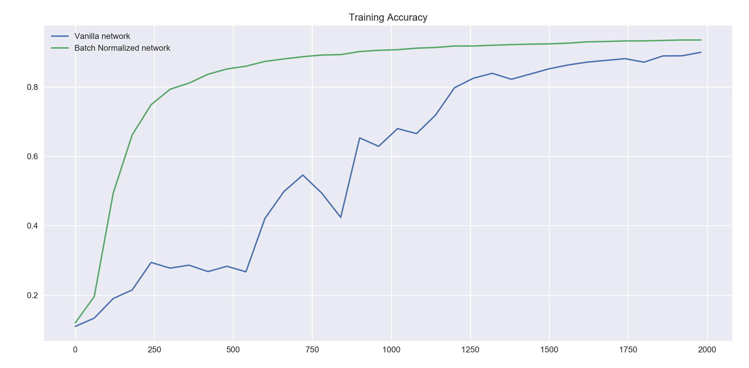
train_network(0.01, 5000, 60, tf.nn.relu, bad_init=True)
 If we use a bad weight initialization strategy with the ReLu non-linearities, even with a small learning rate our vanilla network does not perform at all. Batch normalization seems to be an effective way to counter a bad weight initialization strategy.
Note how the accuracy of the vanilla ReLu network does not seem to change at all. ReLu networks sometimes suffer from units dying out mid training. It is highly likely that this is what we're seeing here.
If we use a bad weight initialization strategy with the ReLu non-linearities, even with a small learning rate our vanilla network does not perform at all. Batch normalization seems to be an effective way to counter a bad weight initialization strategy.
Note how the accuracy of the vanilla ReLu network does not seem to change at all. ReLu networks sometimes suffer from units dying out mid training. It is highly likely that this is what we're seeing here.
Batch normalization doesn't just guard us from an ill-specified model with suboptimal hyperparameters, it maximizes the performance that a good model can give us.
The mechanics of model inference when using batch normalization are slightly different. Instead of using the batch mean and variance, we need to use the population mean and variance when performing inference. These statistcs are kept updated by the context:
with tf.control_dependencies(tf.get_collection(tf.GraphKeys.UPDATE_OPS)):
    optimizer = tf.train.GradientDescentOptimizer(learning_rate).minimize(cross_entropy)
When we're done training and want to use our batch normalized model for predictions, we need to specify to the computational graph that we're not training. This is achieved by passing in the value of the is_training placeholder as False in the feed_dict.
This way, instead of using the per batch mean and variance which would throw off our general predictions, we use population mean and variance that give us the correct predictions.